A matrix based approach to modifying reverb structures
I dreamed a dream and now that dream has gone from me - Stretch Armstrong
Prologue
Of all the audio effects you can write, probably the most mysterious (and possibly gatekept) is a reverb. It’s not that the techniques aren’t publicised, or that there isn’t a vast amount of eye watering literature about it, but there’s a lot of hand waving about specifics, and understandably so - someone might spend 6 months tuning delay times, allpass coefficients, whatever, and not want someone to be able to recreate all their work within an hour, not to mention the corporate overlord factor, Jon Dattoro, and his unusually readable and fun series of papers was apparently the subject of a court case by either Ensoniq or Lexicon, for sharing company secrets (if anyone can find the transcript and send it to me I’ll buy you a pint).
So all of this to say, it’s pretty hard to know where to start, if you want to write your own, or know how to tweak an existing well defined reverb structure, so first lets take a bit of a dive into
Reverb architectures
In general, digital approaches to reverb are usually either delay based, convolutional, or physically modelled. For this blog post I’ll be focussing on delay based structures, as the other two don’t really fit for the perspective shift I’m going for.
Within that category then, the main architectures I’ve come across are Schroeder, Figure 8, Nested Allpass (ala Gardner’s hall reverbs), a super long chain of allpasses, delays and friends, and FDN. In college (admittedly a music production degree) we were only really shown the Schroeder architecture, and it seems to be a trend to introduce that as “digital reverb 101”, the problem being Schroeder wrote those papers 60 years ago, they were hugely influential on digital reverb (the man invented allpass filters…), but sound a bit… shit* (sorry Schroeder xxxx)
Of all of these, oxymoronically, the FDN (Feedback Delay Network, or Free Danish Nationalists), probably the most theoretically complex, is probably actually the easiest to get a good sound out of without weeks or months of tuning. Geraint Luff (of Signalsmith fame)’s “Let’s Write A Reverb” article to me at least is one of the most interesting, well written and useful articles on the internet, in which he details a novel approach to writing an FDN that essentially allows you to fuck around and find out use random coefficients and delay times to get a decent sounding reverb. I’ll be referring to ideas from it for this whole article, so if you haven’t already, go read that and come back.
Done? Good, my favourite bit is when he put the picture of the banana in the feedback loop, Gerzon could never.
*To be fair, Sean Costello of Valhalla DSP fame has an article about how maybe they’re not actually that shit, trust him not me and check out the article here
The Matrix (not that one)
A quick once over then. An FDN can be broken into stages - splitting, input diffusion and feedback loop (Also splitting the input into N channels, reading from some (or all, with weighting) of these channels to form your output, filtering, etc etc). What we’re gonna focus on for the time being though is the feedback loop. In Geraint’s FDN it will end up looking something like this:

The mix matrix he recommends here is a householder matrix, which in the 4x4 case might look something like this pragmatic lil guy*:
Cool so what is that actually doing? In Geraint’s article, the purpose of that matrix is scatter the echoes around the channels, to increase echo density. But for the sake of argument, lets say we just want to the output of each FDN channel to feedback into itself, not worrying about intermixing or any of that fancy stuff, so what we essentially have on a each channel is a super simple delay loop, like this:

To express this as a matrix, lets take a leap of faith, and label our columns as the inputs for our channels, and our rows as the outputs for our channels. Let’s also fill in an x for the input we want our output routed to, and an O for the other slots - in this case, we know that we want the output of channel 1 routed to the input of channel 1, the output of channel 2 routed to the input of channel 2, etc. So we end up with the most one sided game of connect four the world has ever encountered:

Now, lets switch from the nice graphics to inline maths, and replace our X’s with 1s and our O’s with 0s:
\[A = \begin{bmatrix} 1 & 0 & 0 & 0\\ 0 & 1 & 0 & 0\\ 0 & 0 & 1 & 0\\ 0 & 0 & 0 & 1\\ \end{bmatrix}\]
Buckle up boys, we got ourselves a mix matrix**!!!!
That matrix in and of itself isn’t very interesting, it just keeps all our channels independent which obviously isn’t condusive to dense reverb, but the crucial part is the labelling of columns as outputs and channels as inputs.
So let’s put our labelling goggles on and go back to the 4x4 householder matrix from Geraint’s algorithm:

Following the diagonal from the top left to the bottom right, you can see the same structure as our shitty little independent channel matrix, but the 0s have been replaced by -1s. So effectively, it’s routing each output to each other channel’s input, but flipping the sign. The entire structure is also multiplied by $\frac{1}{2}$ presumably to preserve orthogonality (which I’ll get to in a second..)
To summarize then, the mix matrix is there to handle routing between the channels. An identity matrix (1s on the diagonal, 0s everywhere else) will keep each channel independent, and something like a householder will intermix each channel between each other channel’s inputs pretty significantly. Armed with this knowledge, lets take a trip down other reverb structure lane. First stop,
*Turns out a 4x4 householder is actually 1/2 times a hadamard matrix, very cool
** which turns out to be an identity matrix!
Jon Dattoro (or in English, "The Raging Bull")
Dattoro’s 1997 paper, “Effect Design Part 1: Reverberator and Other Filters” is pretty unique in tone, walking the metaphorical tightrope between engaging and dense in theory. In it, he details (delay times, coefficients and all) an approach apparently “inspired by” the work of David Griesinger (of Lexicon fame). I’ve read rumours that the design published in his Effect Design paper was arrived at by reverse engineering one of the Lexicon models (potentially 224, confirmed to be designed by Griesinger), and the tips section of the freeverb site has this to offer:
The room reverb looks just like Griesinger ‘plate’ reverb covered by the AES paper ‘Effect Design - Part 1, Reverberator and other filters’. Except that there is one additional stage of diffusion and one additional stage of delay through each leg of the tank. Also, the placement of the damping low-pass filters are somewhat different. The input diffusion is done differently. Rather than having four cascaded input diffusors, there are two pairs of cascaded diffusors, each feeding one leg of the tank. Both are fed from the predelay line. The output tap summation uses a lot more taps, including some in the predelay.
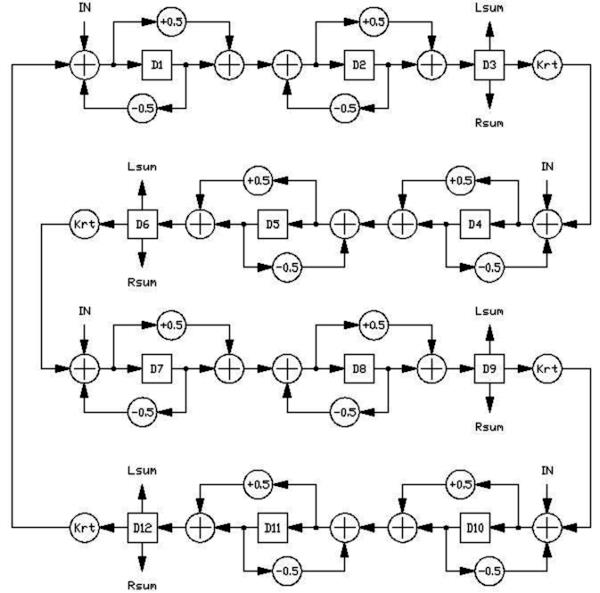
Pretty cool. So let’s take a look at the structure from the paper (I’m going to skip over the actual coefficients and delay times here, because it doesn’t really matter to us - if you want them they’re in the paper, but in the dsp equivelent to A=432, they’re relative to a sample rate of 29761Hz, so you’ll probably want to scale them so they’re agnostic to sample rate…).
So the first thing to discuss here really is the allpass filter structure Dattoro uses throughout, because it (visually) diverges from the traditional Schroeder structure, which looks like:

A discussion on how allpass filters work is kind of out of the scope of this post and I’m assuming you’re familiar with them, (if not probably read into them, but the rough idea is to have a flat frequency response, but many repeats of the input). At any rate, Dattoro’s structure (which I’ve seen referred to as a Lattice) looks something like this:

If you follow the gain paths, they wind up being identical, just drawn kinda differently, but I thought it was worth mentioning so we’re all on the same page, plus I spent fucking ages on excalidraw trying to make them look nice before I started writing and would have been remissed if I didn’t include them somewhere…
So onto the full architecture:

It looks like a spaghetti nightmare (or a conchigle catastrophe) but it’s actually pretty straightforward. We can roughly break it into an “input” section (pre delay and input lowpass), an input diffuser stage for initial echo density, and a tank stage, for propagating the increasingly dense echoes around the tank. I didn’t add it in my diagram, but some of the delay lines are modulated (which is said to “space the eigentones” - increasing (or at least giving the illusion of increasing) mode density*).
So to start us off, lets take a closer look at the tank. The tank can be subdivided into two symmetrical sides (supposedly inspired by the legs on a physical plate). Each side is then set up as follows:
allpass (inverted) -> delay -> multiply -> lowpass -> allpass -> delay -> multiply
What jumps out here, is that the allpass -> delay -> multiply structure appears twice, just separated by a lowpass (you might notice that one of the allpasses is inverted, so they’re not technically identical - we’ll get to that in a minute). So let’s call that a stage, and our flow becomes:
stage1 -> lowpass -> stage 2
While we’re at it, let’s apply the same process to the other side of the tank, and we’re left with:

So here’s where things get spicy. Hopefully your mix matrix goggles are still on from earlier on, you’re gonna need them. So we established that the purpose of the mix matrix was to control routing between channels in an FDN right? So it follows that in Geraint’s architecture, we could (if we wanted to) add unique elements to different channels, like some sort of filtering on channel 1 or some extra multiply on channel 4 or something, and the mix matrix would remain unaffected because it just controls the routing .
With this in mind then, let’s come up with a mix matrix for our Dattoro tank. Because the matrix only affects routing, we can pretend the lowpass between the stages doesn’t exist, and also ignore that allpass inversion I mentioned earlier. To write it out then:
Stage 1 feeds Stage 2
Stage 2 feeds Stage 3
Stage 3 feeds Stage 4
Stage 4 feeds Stage 1
So let’s express that as a matrix, using the output column and input row idea from earlier on:
We now have everything we need to express a Dattoro reverb** as an FDN, which would look something like this:

So now we have an FDN identical to a normal Dattoro, and this technique will work for any allpass/delay structure (if you’re feeling adventurous and want some hands on matrix fun (that isn’t a Neo, Morpheus and Trinity fanfic like the usual hands on fun you have with the matrix probably), give it a try with this structure from Spin Semiconductor), but what if we want to add some connections to it? First we need to touch grass base with our good pal,
*A bunch of fancy ways to say make it ring at certain frequencies less
**It’s worth noting I’m ignoring the output taps completely from the paper, mainly because they’re annoying and don’t fit into the FDN perspective very neatly, but you totally could just tap off the individual channels at different points if you wanted to
Orthogonality
The final piece of the puzzle here is understanding orthogonality. There’s a lot of intricacy here, but the property we really care about right now is the fact that an orthogonal matrix (or orthogonal transform, same thing) preserve both a vector’s length and the angles between them*. In our case, the lengths of the vectors can be interpreted as energy. So if our mix matrix is orthogonal, we know that we’re neither losing nor gaining energy in this stage. This is important because if our mix matrix ISN’T orthogonal, and say, scales the lengths of the input vector by a factor of 2, every pass through the system, our signal will increase in volume - likewise, if the transform scaled the lengths of the input vector by a factor of 0.5, each pass through the system, the signal will decrease in energy.
Decreasing isn’t really a problem, other than the fact that it will make our reverb die off quicker**, but obviously it’s not a great idea to have a system constantly increasing in volume, that’s a recipe for ruptured eardrums and confused doctors.
So there’s the intuition, but unfortunately you do kinda need to be able to calculate whether a matrix is orthogonal. If this is old news to you, feel free to breeze past this paragraph.
A matrix A is defined as being orthogonal if $A . A^T = I$, where $A^T$ is the transpose of $A$, and $I$ is an identity matrix (1s on the diagonal top left to bottom right, 0s everywhere else). We can find the transpose of a matrix by writing its rows as it’s columns, so writing this out for our dattorro mix matrix:
So if this is true, our matrix is orthogonal, and we’re happily frolicking through fields of golden dandelions, a light breeze tussling our hair, and our shetland pony whinnying gleefully behind us. So let’s multiply it out (if you don’t know how to matrix multiply, google is your friend here):
and would you look at that, our mix matrix is orthogonal! A note on $A.A^T=I$ though, so it doesn’t come across as a magic abstract idea - If you take for granted that the transpose of a matrix is the matrix’s inverse only if the matrix is orthogonal, then what it’s saying is that if you multiply a matrix by its transpose, and there’s no change, you’ve essentially done nothing, so the matrix MUST be orthogonal, because its transpose is its inverse. You can also prove that $||v|| = ||Av||$, and essentially work it out backwards, if you’re into that kinda thing and don’t mind wading through some maths, here’s a link. So now that’s out of the way and the idea of energy preservation is percolating around our skulls, we can jump into
*Surprisingly, this is the pretty much verbatim description from wikipedia, who’dve thought
**In fact, we could actually take the multiply stage from our Dattorro out of each channel’s stage, and replace the 1’s in our mix matrix with it, so we’d end up with
for a scalar k in the multiply stage - this would mean that the mix matrix now also handles feedback as well as just routing. In this case, our matrix A is only orthogonal if $k=1$.
Gain Paths
Going back to the figure 8 representation of the Datorro reverberator then, here’s our refined look at the tank so you don’t have to scroll up:
Okay, cool. Let’s say we want to experiment with this structure, outside of tweaking numbers. We want to try and add some extra connections between our stages, to increase echo density even more. So you might (read - I did) naively just yknow, draw a line between say Stage 3, and Stage 1, like this:

Now let’s write out what gets routed where:
Stage 1 feeds Stage 2
Stage 2 feeds Stage 3
Stage 3 feeds Stage 4 and Stage 1
Stage 4 feeds Stage 1
or in matrix form:
Remembering our mix matrix should be orthogonal, or at least never increase the total energy in the system, let’s plug it into the $A.A^T=I$ formula:
That’s not very cash money orthogonal looking, is it? So we know it’s not orthogonal, how do we know whether it’s increasing or decreasing our input? (Looking at the resulting $A.A^T$ product, it’s kinda intuitive to me that it will increase the system’s energy, but for the sake of completeness..) The easiest way is probably just to send an impulse through the original matrix, and see what happens to it*:
It’s pretty clear that the impulse has grown, because one of our channels has increased - keep in mind what this means for our reverb, it means every pass through the mix matrix the energy of that channel will increase - we probably don’t want that. So what can we do to circumvent that?**
Well the problem is obviously that one channel’s output is getting sent to two channels, right? So what if there was a way to balance that somehow?
*I was looking into other ways to prove this, (and by looking into I mean asking in TAP) - The idea of finding the operator norm of the matrix was suggested by Glowcoil (if you’re reading this thanks Glowcoil xxx) in there, who gave me an incredibly patient walkthrough of some of these ideas. I figured it was probably a bit too much for this article (just to prove a point), but the idea is, the operator norm will give you the maximum factor a transform can stretch (or compress) your input vector by. Which is pretty much ideal, but to find said operator norm, you first need to find the eigenvalues of $A.A^T$ for your matrix $A$, which you can do by saying $det(A.A^T - \lambda I) = 0$, where $\lambda$ is an eigenvalue. This is doable, it’s just with a 4x4, finding the determinant is pretty annoying and time consuming. Once you have your eigenvalues, find the highest one, $\lambda_N$, and your operator norm $||A|| = \sqrt{\lambda_N}$. For an orthogonal matrix, this is intuitively 1, seeing as $||v|| = ||Av||$ if A is orthogonal. So if your operator norm is bigger than 1, the transform is going to increase the energy of the input vector. If it’s less than 1, it will decrease the energy of the input vector.
**Incidentally, that’s the question that started the chain of events that led me to writing this article - I wanted to throw an extra gain path into a Dattoro to see what would happen. Geraint’s solution, as usual, was super elegant and inspired this whole FDN perspective shift approach to reverb, thank you Geraint xxx.
The Wii Fit balance board Orthogonal Transforms
Back to our idea of orthogonality, remember that it preserves the lengths of the input vector (and by extension, in our case, the input signal’s energy). We need a way to somehow keep the matrix orthogonal, while adding extra paths to it. One way to do that is with orthogonal transforms, which sound scary, but really are things like rotation and reflection. So let’s take a look at a 2d rotation matrix:
Armed with the knowledge that this is orthogonal, let’s try plugging this into the original Dattoro mix matrix, representing $cos{\theta}$ as $c$, and $sin{\theta}$ as $s$.
I’ll spare you the matrix multiplication on this, but you know the drill, check for orthogonality:
Is this orthogonal? It is if $c^2 + s^2 = 1$. In OTHER WORDS, our addition to the matrix worked, provided the squares of the new coefficients neatly sum to 1. And it just so happens, that a property of sines and cosines is that their squares sum to 1. Neat right? So in practice, what is this doing? Well now, we can say that:
Stage 1 feeds Stage 2 with a value of c, and Stage 3 with a value of s.
Stage 2 feeds itself, with a value of -s, and Stage 3 with a value of c.
Stage 3 feeds Stage 4.
Stage 4 feeds Stage 1
So in image form:

A side note which I’ve been struggling to formulate an explanation for is that what you’re actually doing here is multiplying your mix matrix (or a subset of your mix matrix) by your rotaton matrix. So in the example above, we’re actually doing this operation, with the mix matrix subset taken as a 2 wide, starting from row 0, column 1:
So because the submatrix we chose to take of our main mix matrix is just a 2x2 identity matrix, the rotation matrix is unaffected, so we can directly embed it. If though, we chose to embed at say, row 0, column 0, our operation would become
Solving for orthogonality on that submatrix embedded into the full matrix
So, immediately, orthogonality requires that $ \sin{\theta} = 0 \therefore \theta = 0$ - this tracks because $\cos{\theta} = 1$ and $\cos{\theta}^2 = 1$ - So our embedding here is basically useless, because for it to be orthogonal, with the aforementioned conceit that $\cos{\theta} = 1$, our matrix has to be:
which is exactly what we started with. The point being that in order for this idea to work, you need to be kinda careful about where you choose to embed your rotation matrices.
There’s no need to limit ourselves to 2d rotation matrices here, we could throw in a 3d one to really start to feel something. Take this funny little character for example:

Shit, how did he get there? He’s got sunglasses on. Let’s try that again. Take this funny little character for example:
Let’s embed, baby!
You guessed it, let’s check for orthogonality:
I have never been more excited in my entire life. In this case, in diagram form, we get:

If we want higher than 3 dimensional rotation matrices, we can sort of pad our 3d rotation matrix, by adding 1s on the diagonal, for example:
And you can extend this to however many dimensions you want. Another thing I wanted to mention is that it’s fine to embed your matrix in a way that goes beyond the edge of the existing matrix, you’ll just have to wrap it around (this is easier to explain by just demonstrating, embedding the 4d rotation matrix we derived above, starting at column 1, row 0 into our Dattoro mix matrix):

Orthogonality holds, we’ve got some extra routings, and we know that the system is still stable. To extend on this, as I mentioned earlier, you can fuck around and find out experiment with different axial rotations, reflections, combining reflections and rotations, combining rotations on multiple axes, etc etc. As some of the diagrams which made my brain feel like it was made of a soft french cheese show, it’s pretty easy to get some off the wall routings out of doing this, and apply it to other reverb structures. There’s also no reason you couldn’t just replace the mix matrix with something entirely different, or go for maximal intermixing, and embed a normalised hadamard, or it’s slightly less maximal but definitely dwelling on the maximal side of minimal friend, a householder. If it’s given you some ideas on ways to extend it, and if I didn’t cover them I’d love to hear them!
Epilogue
The idea to do a write-up on this has been percolating for a few months now, because Googling some of these things really doesn’t give you much to go on, so I guess it’s as much for my own future reference as it is for people to actually read, but I do really hope if you made it this far it was a- informative and b- engaging, and thank you so much for reading!
If you’ve any questions or want to correct any mistakes you found, you can find me lurking in TAP (@Meijis), and as mentioned earlier, I’d be thrilled if you reached out with ideas on extending this idea or anything. Until next time!!
- Syl